OpenAI Scholars: First Steps
I am very fortunate to have the opportunity to spend this spring delving into deep learning through the OpenAI Scholars Program. My excellent mentor is Johannes. This is a draft syllabus for the first half of the program, and the current post is a reflection on my first baby steps in AI.
My first few days have been a whirlwind of studying, coding, and highly educational “water cooler conversation”. To paraphrase James Gao, the amount of learning feels like it parallels “early child development”.
Here are some nuggets of insight that I found exciting in my first week. Please note that they are simply my personal observations of things that I didn’t know or hadn’t thought about before I joined this program. If you have related pointers or resources, I’d love to hear about it!
Interpretability was a thing in 1986
Look at this figure from one of the earliest backpropagation papers (Rumelhart et al., 1986, link):
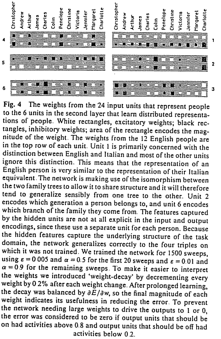
(And if you’re interested in how backpropagation works, I recommend this blog post.)
More recently, feature visualization comes in color. Check out this beautiful work from OpenAI’s Clarity team.
Language models work for reasons
Language models predict the next word (or “token” in a more general sense) given a sequence of words. (See this neat blog post for an illustrated introduction to several recent language models.) It turns out that the performance of language models can tell you something about what type of information a model has learned about the world.
Consider this sentence: “John opens his suitcase and XXX it with clothes”. If the model is able to suggest the word “fills” (a verb in third person singular), this suggests that the model has learned something about grammar.
Now consider this sentence: “Kate could not fit the trophy into her suitcase, because it was too large.” If the model can infer that “it” refers to the trophy rather than the suitcase, this suggests that the model has learned something about physics. Or we can say that it has “learned something about physics” in a very loose sense: Since the model learns from correlations in language, we don’t have reason to believe that it actually has any sort of deep understanding of size in the real world.
I thought the idea was pretty cool.
For those of you who enjoy parallels between artificial and biological neural networks, I recommend checking out neuroscience work on the N400 potential by Marta Kutas (link to wikipedia, link to review paper). This work shows that low-probability words in a sentence elicit a negative-going EEG deflection at about 400 ms after the surprising stimulus. For example, the sentence, “He locked the door using his key” would elicit less of an N400 than the sentence, “He locked the door using his elephant.”
Selection of batch size is kind of a topic…
I was working through a very introductory pytorch tutorial, the 60-minute blitz, and specifically a tutorial on training a “simple” classifier on the CIFAR10 image dataset. Having completed the first learning step of just re-typing each command into my own jupyter notebook and executing it, I wanted to change some variable to see what would happen. I chose “batch size” (without having much understanding of what that is). I updated the batch_size from 4 to 64 training examples. Performance dropped dramatically.
“What is up?”, I wondered, and went through the script line by line. It turns out that, since CIFAR10 has 50,000 training examples and 50,000%64=16, the last batch had only 16 training examples. “Maybe the batch size needs to be a factor of the training set size?” I thought, and proceeded to make my way to the metaphorical water cooler at OpenAI (it’s actually more of a general kitchen area with snacks). Naturally, I ran into another hungry colleague, and inquired about my conundrum. “Oh batch size?” It turns out that he was rather interested in batch sizes, and I ended up with a reference to this blog post and this paper. So batch size selection is quite the topic! I am yet to fully absorb these materials, but some basic information about batches goes as follows:
- When training neural networks, you typically update their weights using a procedure called gradient descent.
- In practice, when you have large datasets, you use a modified version of gradient descent, called stochastic gradient descent (SGD). The word “stochastic” makes this seem scarier than it is: All it means is that you don’t update your model using all of your training data at once. Instead, you select a subset of your training examples, and update the gradient of your model using just those examples. The training examples that you choose is your batch and the number of training examples is your batch size. The “stochastic” part refers to the fact that the gradient directions will have some amount of noise when you use a smaller batch size.
- How big should your batch size be?
- My first-order understanding, which I think is useful as a first way of thinking about it, was the following:
- If you only consider your model performance, it would be best to choose your entire training set, since this will give you the most stable gradient estimate.
- Consider the opposite extreme, where you select a batch size of 1. In this case, you would update your weights based on just a single training example. The gradient would get quite noisy, and your network weights would start hopping back and forth based on the whims of individual training examples.
- Why not use your entire training set? Because it can get very computationally costly if you have a lot of data. This is the reason why we have SGD in the first place. Often a smaller number of training samples is enough to get good model performance. That “good-enough” number of training examples is referred to as the “Critical Batch Size” in the aforementioned blog post.
- My updated understanding after discussion with my mentor is the following:
- Even from a model performance perspective, it can be desirable to have some amount of noise in your gradient updates. This actually helps with finding good parameters. So introducing some noise by having a small batch size can be useful quite separately from the computational gains of SGD. Full gradient descent is more prone to overfitting than SGD.
- The “critical batch size” may only apply to generative language models, and may not generalize to supervised learning, as in my CIFAR10 exercise.
- My first-order understanding, which I think is useful as a first way of thinking about it, was the following:
In the end, it turned out that my particular batch size conundrum was caused by a typo in how I calculated the loss on the test data. But I’m very happy about my serendipitous batch size detour!
You can descend a gradient with respect to the input (rather than the weights)
When I think about gradient descent, I typically think of a picture like this. Some version of this picture is shown in most introductory machine learning and data science classes. It shows the loss function (the curved sheet) as a function of weights (the axes on the bottom) in a simple neural network, with just two weights. We want to update our weights so that we find the bottom (minimum) of this loss function. That’s a basic intuition for gradient descent.
Now assume that we’re doing gradient descent on a really shallow network, also known as a linear regression, with just two weights just like in the figure. Let’s also assume that we use mean squared error as our loss function. Our loss is calculated like this:
…where y is the true labels for the data examples and y-hat is the labels that our models predicted. (N is the number of training examples, but that’s less important for the moment.)
So far, we can see that the loss is a function of the true labels and the predicted labels. How does this relate to the snazzy plot that we started with? We got the predicted labels in some way, specifically like this:
…where X is a matrix of data, which will have the dimension Nx2. w is our weight vector, which will have the dimension 2x1. b is our bias vector, which will have the dimension 2x1. (Notice that the bias is a parameter of the model, just like the weights, and it is usually updated along with the weights.)
What gives? Our loss function actually seems to depend on a few things:
- The parameters, w and b, which are the things that we update, and the things that I had usually thought that the loss depends on.
- But also the data, X, and the labels, y.
It turns out that we usually don’t hear about the loss depending on the data and the labels, because we take those as fixed. But importantly, you can mathematically compute the gradient with respect to the data. You could turn the situation upside down, and assume that you have a network that is already trained, so you take its weights as fixed. Then you could see how some downstream value in the network, such as the activation of a given neuron, changes as you make a small update to the stimulus. And that’s when you start to get into the exciting field of interpretability.
Meta-thoughts on the learning process
Learning to see
If you’re trying to study some math topic in your “free time” during your neuroscience PhD, it can be frustrating to run into the following phrase in a textbook: “It can easily be seen that…” (Mathematicians seem to love using this kind of expression, along with “Proving [X] will be left as an exercise to the reader.”)
Let us pause to reflect on the expression “It can easily be seen that…” In the context of math, the author probably equally intended to say “It can easily be understood that…”. I would like to claim that we should not assume that things can “easily” be understood or even literally seen in a visual sense, unless the reader has practice with understanding or seeing that exact thing or very similar things.
One of the things I’m really interested in understanding during my time at OpenAI is language models, and especially transformer networks. I was pointed to this excellent blog post, which walks you through the first transformer paper and provides a complete code implementation in pytorch.
My first stumbling block was this intimidating diagram:
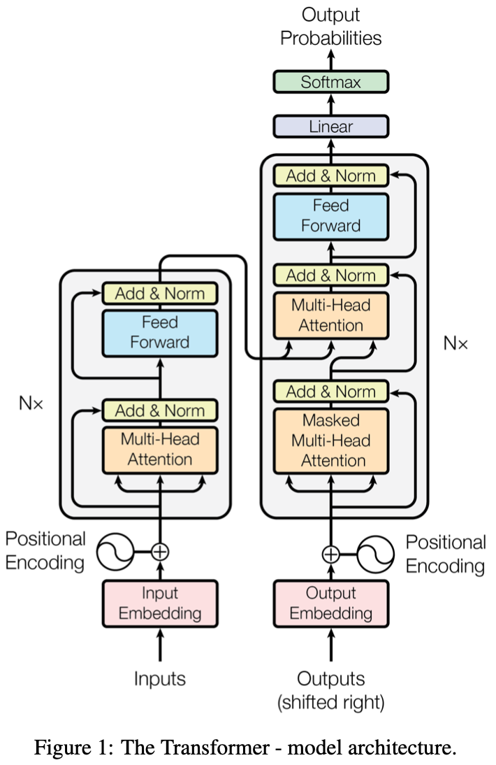
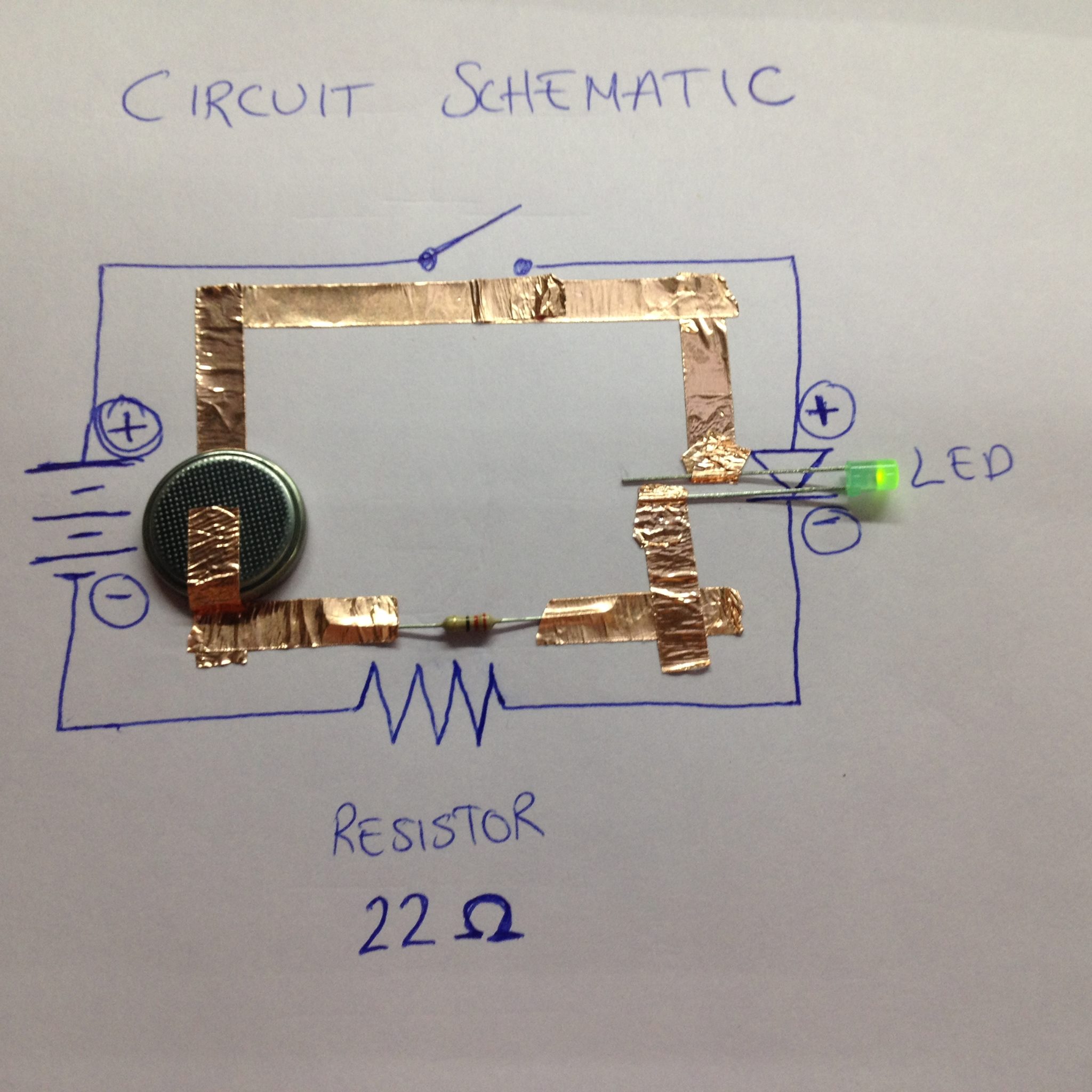
Looking at this, I realized that I have virtually no experience looking at neural network architectures, and very little experience even with other circuit diagrams. (I did dedicate some deliberate practice to learning to see electrical circuit diagrams at one point during my PhD, with great help from a course at the Crucible in Oakland):
Returning to the intimidating transformer diagram:

I realized that I have virtually no (cognitive or mental) tools for understanding this type of image, and what was worse was that I seemed to avoid looking at it at all. For example, I’m pretty sure that I’m literate, so if you had shown me the image and then covered it, and asked me “Was the word ‘multi-head’ in it?” I should have been able to answer you. But I don’t think I would have been. There is nothing in particular preventing me from being able to read that word. But the fact that I knew that this is a type of image that I don’t know how to look at, made me avoid looking at it at all. When I identified this mental blocker, I decided to draw a copy of the diagram, in order to force my brain to take in whatever information that it could take in, and to overtly raise questions about parts that were confusing. My drawing looks like this:
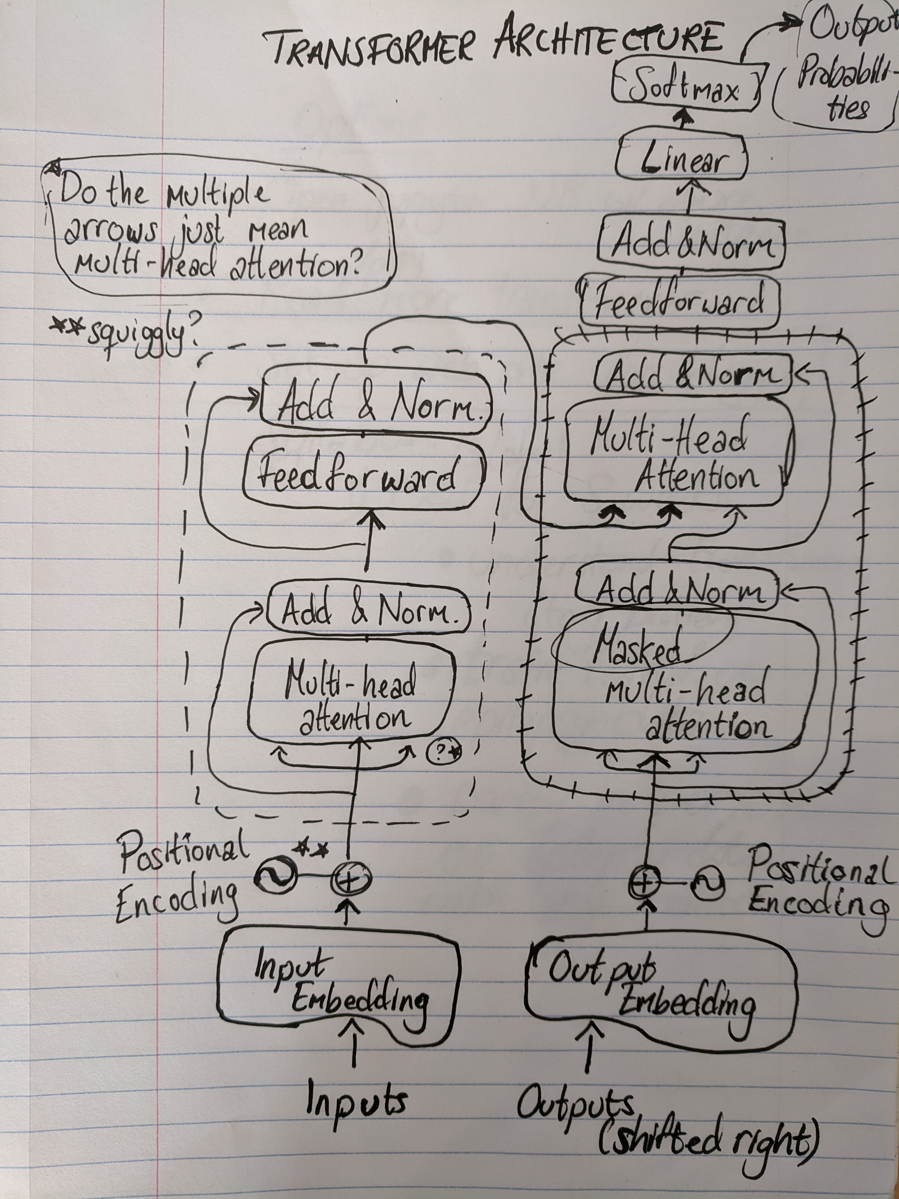 This exercise, along with a set of really nice supplementary materials like this blog post and these videos (video 1, video 2), enabled me to start to break the diagram apart. At this point I could probably tell you a little story about what each part of the architecture is doing. For example, in retrospect, “squiggly” means that the authors of the paper used sine and cosine waves to encode the position of the tokens, since transformer models - unlike recurrent neural networks (RNNs) - don’t natively have any sort of concept of the ordering of tokens in a sequence. We’re becoming more friendly with each other, the diagram and I.
Learning to remember
Continuing on the annotated transformer blog post, I found that belaboring the diagram in detail was helpful in a way, but it also had me neglect the rest of the blog post. It seemed like it would be useful to at least get an overview of what’s in there, without spending an unreasonable amount of time on every single paragraph and line of code (googling terms and commands and going off on every possible tangent of things I don’t yet know). So I decided to read the whole post once without stopping. Then I wrote down what I could remember of what I had read. That exercise went approximately like this:
I took a speed-reading course and read War and Peace in twenty minutes. It involves Russia.
(Woody Allen)
In fact, the only parts of that read that I could recall were things that my mentor, Johannes, had specifically pointed out to me (verbally) before. So that was interesting. It seems like it would be a good idea to deliberately hack what sort of things enable you to remember and understand, and to be able to apply them more quickly and efficiently. So this is an open question for you, dear reader:
Do you have learning hacks that allow you to quickly understand and remember new information?
By the way, if you’re interested in the processes of “looking” and “remembering”, it turns out that they might be highly related from a neural perspective (link to exciting paper by Miriam Meister and Beth Buffalo).
That’s all I have for now. By next time, I hope to have run into more problems in the space of coding and implementing neural network architectures.